The price of an option, known as its premium, is influenced by various factors, including the current market price of the underlying asset, the strike price, the time remaining until expiration, implied volatility, and interest rates. Option pricing models aim to quantify the fair value of an option based on these factors. The formula for calculating the theoretical price of a European put option is a modification of the call option formula.
Key Components
Introduction to Option Pricing
Options are a type of financial derivative that derive their value from an underlying asset, such as stocks, bonds, commodities, or currencies. There are two primary types of options:
Key Option Pricing Models
Several models have been developed over the years to calculate the theoretical value of options. The two most widely used option pricing models are:
Factors Influencing Option Prices
Several key factors influence the pricing of options:
Real-World Applications of Option Pricing
Option pricing models are used in various real-world applications, including:
Limitations of Option Pricing Models
While option pricing models are valuable tools in finance, they have certain limitations:
Conclusion
Option pricing is a critical concept in finance, enabling investors, traders, and financial institutions to determine the fair value of financial options.
Strengths
—
Limitations
✗Assumptions: Option pricing models, including the Black-Scholes model, rely on simplifying assumptions, such as constant volatility and…
✗Market Behavior: Option pricing models assume that market prices follow a random walk or geometric Brownian motion.
✗Transaction Costs: Option pricing models often do not account for transaction costs, which can significantly impact trading strategies.
✗Dividends: The treatment of dividends in option pricing models can be complex, especially for American-style options on dividend-paying…
✗Market Liquidity: The availability of options with different strike prices and expiration dates can vary, affecting the practicality of…
When Not To Use
▲Assumptions: Option pricing models, including the Black-Scholes model, rely on simplifying assumptions, such as constant…
▲Market Behavior: Option pricing models assume that market prices follow a random walk or geometric Brownian motion.
▲Transaction Costs: Option pricing models often do not account for transaction costs, which can significantly impact trading…
▲Dividends: The treatment of dividends in option pricing models can be complex, especially for American-style options on…
Quick Answers
What are the key option pricing models?
Several models have been developed over the years to calculate the theoretical value of options. The two most widely used option pricing models are:
What is Real-World Applications of Option Pricing?
Option pricing models are used in various real-world applications, including:
What are the limitations of option pricing models?
While option pricing models are valuable tools in finance, they have certain limitations:
Key Insight
Option pricing is a critical concept in finance, enabling investors, traders, and financial institutions to determine the fair value of financial options. The two primary option pricing models, the Black-Scholes model and the binomial model, provide frameworks for calculating option premiums based on factors such as the current market price of the underlying asset, strike price, time to expiration, implied volatility, and risk-free interest…
Exec Package + Claude OS Master Skill | Business Engineer Founding Plan
FourWeekMBA x Business Engineer | Updated 2026
Option Pricing Model / Component
Type
Description
When to Use
Example
Formula
Black-Scholes Model
Model
A mathematical model used to calculate the theoretical price of European-style options (calls and puts).
Valuing European options with known volatility and interest rates.
The Black-Scholes price of a call option is $10.
Black-Scholes Formula
Binomial Option Pricing Model
Model
A discrete-time model used to calculate option prices by creating a binomial tree of possible price movements.
Valuing American-style options and options with early exercise features.
The binomial price of a put option is $8.
Binomial Option Pricing Formula
Option Greeks (Delta, Gamma, Theta, Vega, Rho)
Sensitivity
Sensitivity measures that indicate how an option’s price changes in response to various factors: Delta (Δ) – Price change in response to the underlying asset’s price change. Gamma (Γ) – Rate of change of Delta in response to asset price changes. Theta (Θ) – Time decay of an option’s value as time passes. Vega (ν) – Sensitivity to changes in implied volatility. Rho (ρ) – Sensitivity to changes in interest rates.
Managing option portfolios and understanding risk exposures.
A call option has a Delta of 0.65, indicating a $0.65 increase for a $1 increase in the underlying asset’s price.
Options are a type of financial derivative that derive their value from an underlying asset, such as stocks, bonds, commodities, or currencies. There are two primary types of options:
Call Options: These give the holder the right to buy the underlying asset at the strike price before or on a specified expiration date.
Put Options: These give the holder the right to sell the underlying asset at the strike price before or on a specified expiration date.
The price of an option, known as its premium, is influenced by various factors, including the current market price of the underlying asset, the strike price, the time remaining until expiration, implied volatility, and interest rates. Option pricing models aim to quantify the fair value of an option based on these factors.
Key Option Pricing Models
Several models have been developed over the years to calculate the theoretical value of options. The two most widely used option pricing models are:
1. Black-Scholes Model:
Developed by economists Fischer Black, Myron Scholes, and Robert Merton in the early 1970s, the Black-Scholes model is considered a pioneering work in option pricing theory. This model provides a mathematical framework for calculating the theoretical price of European-style options (options that can only be exercised at expiration). The Black-Scholes formula takes into account the following variables:
Current market price of the underlying asset (S).
Strike price of the option (K).
Time to expiration (T).
Implied volatility (σ), which represents the expected future volatility of the underlying asset’s price.
Risk-free interest rate (r), typically based on the yield of a risk-free government bond.
The Black-Scholes formula for calculating the theoretical price of a European call option is as follows:
plaintextCopy code
C = S * N(d1) - K * e^(-rT) * N(d2)
Where:
C is the call option’s theoretical price.
N(d1) and N(d2) are cumulative probability functions.
e represents the base of the natural logarithm.
The formula for calculating the theoretical price of a European put option is a modification of the call option formula.
2. Binomial Option Pricing Model:
The binomial option pricing model is a more versatile approach that can be applied to both European and American-style options (options that can be exercised at any time before or on the expiration date). Unlike the Black-Scholes model, which provides a closed-form solution, the binomial model uses a tree-based framework to approximate option prices. The key components of the binomial model include:
Current market price of the underlying asset (S).
Strike price of the option (K).
Time to expiration (T), divided into discrete time intervals.
Implied volatility (σ).
Risk-free interest rate (r).
The binomial model works by constructing a binomial tree that represents possible price movements of the underlying asset over time. At each node of the tree, the model calculates the option’s value based on the probability of the asset’s price moving up or down. The model then uses a backward induction process to determine the option’s fair value at the initial node (today’s date).
Factors Influencing Option Prices
Several key factors influence the pricing of options:
1. Current Market Price of the Underlying Asset (S):
The price of the underlying asset plays a significant role in option pricing. For call options, as the underlying asset’s price increases, the option’s value generally increases. Conversely, for put options, as the underlying asset’s price decreases, the option’s value typically increases.
2. Strike Price (K):
The strike price is the price at which the option holder has the right to buy (for call options) or sell (for put options) the underlying asset. The relationship between the strike price and the current market price of the underlying asset affects option pricing. In general, call options with strike prices below the current market price of the underlying asset (in-the-money) have higher premiums, while put options with strike prices above the current market price (in-the-money) also have higher premiums.
3. Time to Expiration (T):
The amount of time remaining until the option’s expiration date impacts its price. Options with more time until expiration tend to have higher premiums because there is a greater chance that the option will become profitable. Time decay, also known as theta decay, erodes the value of options as they approach their expiration date.
4. Implied Volatility (σ):
Implied volatility represents the market’s expectation of future price volatility of the underlying asset. Higher implied volatility leads to higher option premiums because there is a greater likelihood of significant price movements, which can result in larger potential profits for option holders.
5. Risk-Free Interest Rate (r):
The risk-free interest rate, typically based on government bond yields, is used to discount the future cash flows associated with options. Higher interest rates lead to higher call option premiums and lower put option premiums.
Real-World Applications of Option Pricing
Option pricing models are used in various real-world applications, including:
1. Investment Decisions:
Investors and traders use option pricing models to assess the fair value of options and make informed investment decisions. They can compare the calculated option price to the market price to determine whether an option is undervalued or overvalued.
2. Risk Management:
Financial institutions and corporations use options to manage risk exposure in their portfolios. Option pricing models help quantify the cost of hedging strategies, such as buying put options to protect against downside risk in a stock portfolio.
3. Employee Stock Options:
Companies often issue stock options to employees as part of their compensation packages. Option pricing models are used to determine the fair value of these employee stock options for accounting and financial reporting purposes.
4. Derivative Trading:
Traders in financial markets use option pricing models to develop trading strategies involving options. They may seek arbitrage opportunities by identifying mispriced options and taking advantage of price discrepancies.
5. Valuation of Complex Derivatives:
In addition to standard call and put options, option pricing models are used to value more complex derivatives, such as exotic options, binary options, and barrier options.
Limitations of Option Pricing Models
While option pricing models are valuable tools in finance, they have certain limitations:
Assumptions: Option pricing models, including the Black-Scholes model, rely on simplifying assumptions, such as constant volatility and interest rates. These assumptions may not always hold in the real world.
Market Behavior: Option pricing models assume that market prices follow a random walk or geometric Brownian motion. In reality, market behavior can be influenced by various factors, including news events, market sentiment, and geopolitical developments.
Transaction Costs: Option pricing models often do not account for transaction costs, which can significantly impact trading strategies.
Dividends: The treatment of dividends in option pricing models can be complex, especially for American-style options on dividend-paying stocks.
Market Liquidity: The availability of options with different strike prices and expiration dates can vary, affecting the practicality of certain trading strategies.
Conclusion
Option pricing is a critical concept in finance, enabling investors, traders, and financial institutions to determine the fair value of financial options. The two primary option pricing models, the Black-Scholes model and the binomial model, provide frameworks for calculating option premiums based on factors such as the current market price of the underlying asset, strike price, time to expiration, implied volatility, and risk-free interest rate. These models have real-world applications in investment decisions, risk management, employee stock options, derivative trading, and the valuation of complex financial instruments. However, they come with limitations and assumptions that should be considered when using them in practice. Understanding option pricing is essential for anyone involved in financial markets and derivative trading, as it forms the basis for informed decision-making and risk management strategies.
The circle of competence describes a person’s natural competence in an area that matches their skills and abilities. Beyond this imaginary circle are skills and abilities that a person is naturally less competent at. The concept was popularised by Warren Buffett, who argued that investors should only invest in companies they know and understand. However, the circle of competence applies to any topic and indeed any individual.
Economic or market moats represent the long-term business defensibility. Or how long a business can retain its competitive advantage in the marketplace over the years. Warren Buffet who popularized the term “moat” referred to it as a share of mind, opposite to market share, as such it is the characteristic that all valuable brands have.
The Buffet Indicator is a measure of the total value of all publicly-traded stocks in a country divided by that country’s GDP. It’s a measure and ratio to evaluate whether a market is undervalued or overvalued. It’s one of Warren Buffet’s favorite measures as a warning that financial markets might be overvalued and riskier.
Venture capital is a form of investing skewed toward high-risk bets, that are likely to fail. Therefore venture capitalists look for higher returns. Indeed, venture capital is based on the power law, or the law for which a small number of bets will pay off big time for the larger numbers of low-return or investments that will go to zero. That is the whole premise of venture capital.
Foreign direct investment occurs when an individual or business purchases an interest of 10% or more in a company that operates in a different country. According to the International Monetary Fund (IMF), this percentage implies that the investor can influence or participate in the management of an enterprise. When the interest is less than 10%, on the other hand, the IMF simply defines it as a security that is part of a stock portfolio. Foreign direct investment (FDI), therefore, involves the purchase of an interest in a company by an entity that is located in another country.
Micro-investing is the process of investing small amounts of money regularly. The process of micro-investing involves small and sometimes irregular investments where the individual can set up recurring payments or invest a lump sum as cash becomes available.
Meme stocks are securities that go viral online and attract the attention of the younger generation of retail investors. Meme investing, therefore, is a bottom-up, community-driven approach to investing that positions itself as the antonym to Wall Street investing. Also, meme investing often looks at attractive opportunities with lower liquidity that might be easier to overtake, thus enabling wide speculation, as “meme investors” often look for disproportionate short-term returns.
Retail investing is the act of non-professional investors buying and selling securities for their own purposes. Retail investing has become popular with the rise of zero commissions digital platforms enabling anyone with small portfolio to trade.
Accredited investors are individuals or entities deemed sophisticated enough to purchase securities that are not bound by the laws that protect normal investors. These may encompass venture capital, angel investments, private equity funds, hedge funds, real estate investment funds, and specialty investment funds such as those related to cryptocurrency. Accredited investors, therefore, are individuals or entities permitted to invest in securities that are complex, opaque, loosely regulated, or otherwise unregistered with a financial authority.
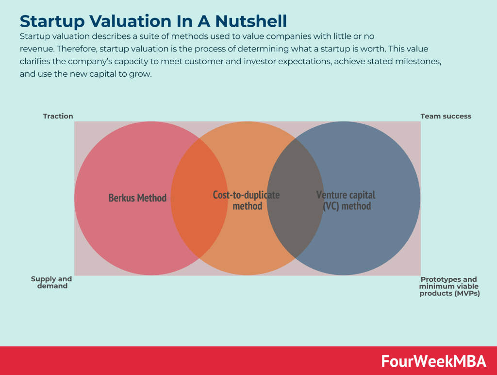
Startup valuation describes a suite of methods used to value companies with little or no revenue. Therefore, startup valuation is the process of determining what a startup is worth. This value clarifies the company’s capacity to meet customer and investor expectations, achieve stated milestones, and use the new capital to grow.
Profit is the total income that a company generates from its operations. This includes money from sales, investments, and other income sources. In contrast, cash flow is the money that flows in and out of a company. This distinction is critical to understand as a profitable company might be short of cash and have liquidity crises.
Double-entry accounting is the foundation of modern financial accounting. It’s based on the accounting equation, where assets equal liabilities plus equity. That is the fundamental unit to build financial statements (balance sheet, income statement, and cash flow statement). The basic concept of double-entry is that a single transaction, to be recorded, will hit two accounts.
The purpose of the balance sheet is to report how the resources to run the operations of the business were acquired. The Balance Sheet helps to assess the financial risk of a business and the simplest way to describe it is given by the accounting equation (assets = liability + equity).
The income statement, together with the balance sheet and the cash flow statement is among the key financial statements to understand how companies perform at fundamental level. The income statement shows the revenues and costs for a period and whether the company runs at profit or loss (also called P&L statement).
The cash flow statement is the third main financial statement, together with income statement and the balance sheet. It helps to assess the liquidity of an organization by showing the cash balances coming from operations, investing and financing. The cash flow statement can be prepared with two separate methods: direct or indirect.
The capital structure shows how an organization financed its operations. Following the balance sheet structure, usually, assets of an organization can be built either by using equity or liability. Equity usually comprises endowment from shareholders and profit reserves. Where instead, liabilities can comprise either current (short-term debt) or non-current (long-term obligations).
Capital expenditure or capital expense represents the money spent toward things that can be classified as fixed asset, with a longer term value. As such they will be recorded under non-current assets, on the balance sheet, and they will be amortized over the years. The reduced value on the balance sheet is expensed through the profit and loss.
Financial statements help companies assess several aspects of the business, from profitability (income statement) to how assets are sourced (balance sheet), and cash inflows and outflows (cash flow statement). Financial statements are also mandatory to companies for tax purposes. They are also used by managers to assess the performance of the business.
Financial modeling involves the analysis of accounting, finance, and business data to predict future financial performance. Financial modeling is often used in valuation, which consists of estimating the value in dollar terms of a company based on several parameters. Some of the most common financial models comprise discounted cash flows, the M&A model, and the CCA model.
Business valuations involve a formal analysis of the key operational aspects of a business. A business valuation is an analysis used to determine the economic value of a business or company unit. It’s important to note that valuations are one part science and one part art. Analysts use professional judgment to consider the financial performance of a business with respect to local, national, or global economic conditions. They will also consider the total value of assets and liabilities, in addition to patented or proprietary technology.
The Weighted Average Cost of Capital can also be defined as the cost of capital. That’s a rate – net of the weight of the equity and debt the company holds – that assesses how much it cost to that firm to get capital in the form of equity, debt or both.
A financial option is a contract, defined as a derivative drawing its value on a set of underlying variables (perhaps the volatility of the stock underlying the option). It comprises two parties (option writer and option buyer). This contract offers the right of the option holder to purchase the underlying asset at an agreed price.What are the key components of Option Pricing?
The key components of Option Pricing include Black-Scholes Model, Binomial Option Pricing Model, Option Greeks (Delta, Gamma, Theta, Vega, Rho), Implied Volatility, Intrinsic Value. Black-Scholes Model: Model Binomial Option Pricing Model: Model
The formula for calculating the theoretical price of a European put option is a modification of the call option formula.
How do you apply Option Pricing in practice?
The binomial model works by constructing a binomial tree that represents possible price movements of the underlying asset over time. At each node of the tree, the model calculates the option’s value based on the probability of the asset’s price moving up or down. The model then uses a backward induction process to determine the option’s fair value at the initial node (today’s date).
What are the advantages and limitations of Option Pricing?
The price of the underlying asset plays a significant role in option pricing. For call options, as the underlying asset’s price increases, the option’s value generally increases. Conversely, for put options, as the underlying asset’s price decreases, the option’s value typically increases.
What are the key option pricing models?
Several models have been developed over the years to calculate the theoretical value of options. The two most widely used option pricing models are:
What are the key components of Option Pricing?
The key components of Option Pricing include Introduction to Option Pricing, Key Option Pricing Models, Factors Influencing Option Prices, Real-World Applications of Option Pricing, Limitations of Option Pricing Models. Introduction to Option Pricing: Options are a type of financial derivative that derive their value from an underlying asset, such as stocks, bonds, commodities, or currencies.
Frequently Asked Questions
What is Option Pricing?
The price of an option, known as its premium, is influenced by various factors, including the current market price of the underlying asset, the strike price, the time remaining until expiration, implied volatility, and interest rates. Option pricing models aim to quantify the fair value of an option based on these factors. The formula for calculating the theoretical price of a European put option is a modification of the call option formula.
What are the key option pricing models?
Several models have been developed over the years to calculate the theoretical value of options. The two most widely used option pricing models are:
What are the key components of Option Pricing?
The key components of Option Pricing include Introduction to Option Pricing, Key Option Pricing Models, Factors Influencing Option Prices, Real-World Applications of Option Pricing, Limitations of Option Pricing Models. Introduction to Option Pricing: Options are a type of financial derivative that derive their value from an underlying asset, such as stocks, bonds, commodities, or currencies. There are two primary types of options:
Gennaro is the creator of FourWeekMBA, which reached about four million business people, comprising C-level executives, investors, analysts, product managers, and aspiring digital entrepreneurs in 2022 alone | He is also Director of Sales for a high-tech scaleup in the AI Industry | In 2012, Gennaro earned an International MBA with emphasis on Corporate Finance and Business Strategy.
Scroll to Top
Discover more from FourWeekMBA
Subscribe now to keep reading and get access to the full archive.


")


