30 Advanced Google Sheets Formulas For Business People
Google Sheets is among the most powerful and free productivity tools for business people. It enables you to create from simple to more complex spreadsheets, with minimum sophistication, and in many cases, with out of the box formulas, that can handle complex tasks and all this in the cloud, therefore your document is always updated, it can be shared easily with other team members and worked upon.
Visual Overview
Key Components
GOOGLETRANSLATE
GOOGLETRANSLATE is a function that has made understanding texts in different languages possible. This function enables the user to translate certain text from one language to the other, so that has broadened the scope of Google sheets.
IMAGE
This function is very simple to use and makes the spreadsheet more appealing. Image is function simply adds a specified image in the cell or range. Following is the syntax.
SPARKLINE
SPARKLINE function enables the users to incorporate mini charts in a single cell of spreadsheets to make them more descriptive and convenient to analyze data . Following is the syntax.
ISBLANK
ISBLANK function determines if a cell is empty or not. This function outputs the value as true if the cell is empty and false if the value is not empty. Following is the syntax.
ISDATE
ISDATE function determines whether a value contained in a cell is a date or not. Following is the syntax.
ISMAIL
ISMAIL function is used to check whether a certain email address provided in the data is valid or not. Following is the syntax.
ISERROR
This function is classified as an information error and it is used to determine an error in a value. Following is the syntax.
ISFORMULA
ISSFORMULA is also classified as an information function. It is employed to determine whether a cell or range contain a formula or not. Following is the syntax.
ISNONTEXT
This function comes in handy when you want to determine whether a cell contains a value, which is not in a textual form such as a date, a number, or time. Following is the syntax.
ISNUMBER
ISNUMBER is the function, which is used to mark numbers in data . Following is the syntax.
Strengths
—
Limitations
✗This function restricts the size of the input arrays and outputs the specified number of rows and columns of that array.
GOOGLETRANSLATE is a function that has made understanding texts in different languages possible. This function enables the user to translate certain text from one language to the other, so that has broadened the scope of Google sheets. Following is the syntax.
What is IMAGE?
This function is very simple to use and makes the spreadsheet more appealing. Image is function simply adds a specified image in the cell or range. Following is the syntax.
What is SPARKLINE?
SPARKLINE function enables the users to incorporate mini charts in a single cell of spreadsheets to make them more descriptive and convenient to analyze data . Following is the syntax.
Key Insight
Here, DATEDIF is the name of this date function. Start_of_date refers to the date from where the calculations should start. It may contain a numeric value, a cell consisting of a DATE, or a function translating into a DATE type. End_of_date indicates the date on which the calculations are to end. Likewise, it may also contain a numeric value, a cell consisting of a DATE or a function translating into a DATE type.
Exec Package + Claude OS Master Skill | Business Engineer Founding Plan
FourWeekMBA x Business Engineer | Updated 2026
Last Updated: April 2026
Google Sheets is among the most powerful and free productivity tools for business people.
It enables you to create from simple to more complex spreadsheets, with minimum sophistication, and in many cases, with out of the box formulas, that can handle complex tasks and all this in the cloud, therefore your document is always updated, it can be shared easily with other team members and worked upon.
Google Sheets is an incredible tool that can also create advanced visualizations, spreadsheets, and handle anything your business might need. And with that in mind, below a set of advanced formulas you can use to grow your own business!
GOOGLETRANSLATE
GOOGLETRANSLATE is a function that has made understanding texts in different languages possible. This function enables the user to translate certain text from one language to the other, so that has broadened the scope of Google sheets. Following is the syntax.
GOOGLE TRANSLATE (text, [source language, target language])
Here GOOGLETRANSLATE is the name of the function. The input contains text, the source language, and the target language. The text refers to the selected text that you want to translate, source language refers to the language from which you want to translate your text, and target language refers to the specific language in which you want to translate your text. There is a two-letter code for source or target language, which should be written within quotation marks. For example, “en” for English and “ko” for the Korean language.
IMAGE
This function is very simple to use and makes the spreadsheet more appealing. Image is function simply adds a specified image in the cell or range. Following is the syntax.
IMAGE (url, [mode], [height], [width])
IMAGE is the name of the function and url refers to URL of the image which must have a protocol as http: / /. Mode refers to the different sizes that the image can have. These modes are used to compress, crop, or make custom size of an image. Height refers to the specific height of the image and it can be customized by using mode 4. The width refers to the width of a particular image measured in pixels and it can also be customized.
SPARKLINE
SPARKLINE function enables the users to incorporate mini charts in a single cell of spreadsheets to make them more descriptive and convenient to analyzedata. Following is the syntax.
SPARKLINE (data, [options])
SPARKLINE is the name of function. Data refers to the range or array in which a chart is to be incorporated. Options refer to the additional setting and options for incorporating charts. There is an option ‘charttype’, which contains a list of charts that can be added. The list contains the line, bar, column, and winloss charts. Colors can also be added and changed in the charts.
ISBLANK
ISBLANK function determines if a cell is empty or not. This function outputs the value as true if the cell is empty and false if the value is not empty. Following is the syntax.
ISBLANK (value)
ISBLANK is the name of the function whereas value refers to the cells that are analyzed under this function for whether they are empty or contain data.
ISDATE
ISDATE function determines whether a value contained in a cell is a date or not. Following is the syntax.
ISDATE (value)
ISDATE is the name of function and value refers to the data in the cell which is to be confirmed as a date. It must be ensured to put the date within quotation marks for the function to output properly.
ISMAIL
ISMAIL function is used to check whether a certain email address provided in the data is valid or not. Following is the syntax.
ISMAIL (value)
Here ISMAIL is the name of the function and input consists of a value which is in the form of an email address and is verified through this function.
ISERROR
This function is classified as an information error and it is used to determine an error in a value. Following is the syntax.
ISERROR (value)
ISSERROR is the name of the function and value refers to the value or values to be checked as error(s). This function is used to check all the errors in spreadsheets. If there is an error then the function outputs as true and if there is no error then the function outputs as false.
ISFORMULA
ISSFORMULA is also classified as an information function. It is employed to determine whether a cell or range contain a formula or not. Following is the syntax.
ISSFORMULA (cell)
ISSFORMULA is the name of the function. The input consists of a cell or range to check if that cell or range includes a formula. The function outputs as true if the cell or range contains a formula and it outputs as false if there is no formula.
ISNONTEXT
This function comes in handy when you want to determine whether a cell contains a value, which is not in a textual form such as a date, a number, or time. Following is the syntax.
ISNONTEXT (value)
ISNONTEXT is the name of the function, the input contains value, which is examined as textual or non-textual value. This function outputs as false if there is text in the cell, and true if there is no text found. An empty cell also outputs as a true value but an empty string outputs as a false value. This function is usually used along with IF function.
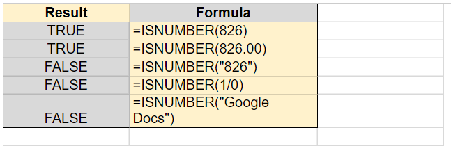
ISNUMBER
ISNUMBER is the function, which is used to mark numbers in data. Following is the syntax.
ISNUMBER (value)
ISNUMBER is the name of the function and input contains a value that is to be determined as a numeric value. The output is true when there is a number in the cell and false when there is no numeric value. This function is also mostly used along with IF function.
ARRAY_CONSTRAIN
This function restricts the size of the input arrays and outputs the specified number of rows and columns of that array. Following is the syntax of this function.
Here the range_of _input is a range of the input data, output_rows is the number of rows that we want in our data, and output_columns is the number of columns that our result may contain. This function is employed along with other formulas when a fewer number of rows and columns are needed in the output.
FREQUENCY
This array function is employed to calculate the frequency of values in a range, known as the one-column range. It gives a vertical array result. The syntax for this function is as follows.
FREQUENCY (data, classes)
Here, datarefers to the range or array with the values that are required to be counted. Classes refer to the range with a set of classes. It should be noted that the classes must be sorted to have clarity. The FREQUENCY will output in the form of a specific vertical sized range one greater than classes. An example of the use of this function is given below.
MDETERM
This function is employed to find out the determinant matrix of a given array. Matrix determinant enables the user to calculate the different qualities of the matrix. It should be noticed that the array must be a square matrix comprising only numbers and not any blanks. Following is the syntax for this function.
MDETERM (square_of_matrix)
Here, square_of_matrix represents an array consisting of an equal number of rows and columns; it is the input of this function. A complete matrix should be the input, which will result in a matrix determinant of that specific square matrix. This function can be employed in mathematics to solve system equations in linear algebra. The example is as follows.
MINVERSE
This function determines the multiplicative inverse matrix of a square matrix. This function works specifically with a square matrix, containing numbers only and comprising equal numbers of rows and columns. Following is the syntax for the function.
MINVERSE (square_of_matrix)
Here, MINVERSE is the name of our function; square_of_matix is the input of this function. This function does not work if the array is empty or if it includes text. It enables among other things to calculate a series of simultaneous equations. Following is an example of the use of this function.
MMULT
This array function enables the user to multiply two matrices classified into ranges or arrays. Following is the syntax for the function.
MMULT (matrix1, matrix2)
Here, MMULT is the name of our function. Matrix1 is the name of the first matrix indicated as range or array while matrix2 is the name of the second matrix also indicated as range or array. For the function to work, the standard must be followed. The standard indicates that the columns in matrix1 must be equal in numbers to the rows in matrix2. The output of this function results in the same number of rows as array 1 and the same number of columns in array 2. An example of the use of this function is as follows.
SUMPRODUCT
This array function multiplies 2 or more corresponding entries of equal-sized arrays or ranges and then determines their sum. This function is pivotal in situations where we need to multiply entries across arrays and determine their sum. Following is the syntax for this function.
SUMPRODUCT (array1, [array2, …])
Here, SUMPRODUCT is the name of our function. Array1 refers to the first array or range whose items are to be multiplied with the items of the second array or range via the SUMPRODUCT formula. Array2 refers to the additional arrays or ranges consisting of the same length as the first array or range. Its entries are to be multiplied with the corresponding entries of the first array or range via SUMPRODUCT. Furthermore, SUMPRODUCT can be paired with TRANSPOSE function, resulting in MMULT.
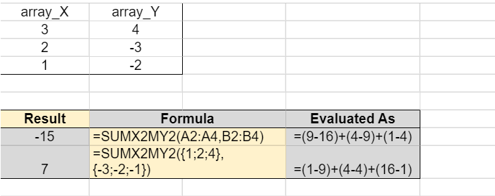
SUMX2MY2
This function enables the user to determine the sum of differences of the entries in two arrays. Following is the syntax for this function.
SUMX2MY2 (array_of_x, array_of_y)
Here, SUMX2MY2 is our function, array_of_x represents the array or range of the entries whose squares are to be minimized by the squares of correlating items in the array_of_y. Then their sum is obtained. On the other hand, Array_of_y represents the array or range of the entries whose squares are to be deducted from the correlating, and then their sum is calculated. An example of the use of this function is shown below.
SUMX2PY2
SUMX2PY2 is an array function that is utilized to find the sum of correlating square entries in two arrays or ranges, which in turn result in sums of their results. It should be noted that the non-numeric values including the text are ignored in the array while using this function. It is used in many statistical problems. The syntax for this function is as follows.
SUMX2PY2 (array_of_x, array_of_y)
Here, SUMX2PY2 is the name of our function. Array_of_x refers to the set of given square entries that are to be added to the square entries of the correlating array or range of array_of_y. While array_of_y refers to the square entries of range or an array whose items are to be added to the correlating square entries of array_of_x.
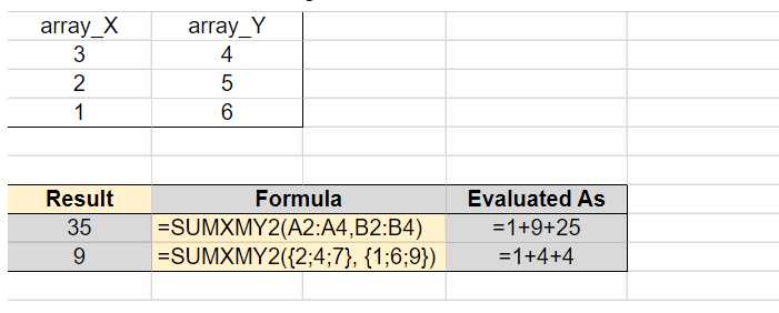
SUMXMY2
This array function enables the user to determine the sum of squares of differences of values in two given arrays. This function outputs a numeric value. Following is the syntax of this function.
SUMXMY2 (array_of_x, array_of_y)
Here, SUMXMY2 is the name of the function, array_of_x refers to the array or range of the entries that are first minimized by correlating items in array_of_y, then they get squared, and finally, these results are summed up. On the other hand, array_of_y represents the range or array of the entries that will first be deducted from the correlating items of array_of_x, and then they get squared, and finally, these results are summed up.
TRANSPOSE
This array function is very useful when the user wants to relocate the column or rows in an array or range of cells in Google sheets. This function can alter the arrangement of spreadsheets from vertical to horizontal or vice-versa. Following is the syntax of this function.
TRANSPOSE (array_or_range)
Here, TRANSPOSE is the name of the function, while array_or_range consists of the columns and rows of array or range, which are required to be interchanged. This transpose function is very suitable for presentation purposes.
DATE
The DATE function is employed when the userneeds to convert the data in the form of DATE from the data that is in the form of a year, month, or day. The syntax for this function is as follows.
DATE (year, month, day)
Here, DATE is the name of this function, a year represents the year section of the date, a month represents the month section of the date, while day refers to the day section of the date. Now certain things should be considered. Firstly, all the input of date should be in numeric form for the function to work properly, otherwise, the output will contain a value error. Further, the DATE is recalculated if the numeric value of the date goes beyond the valid month or day range. For example, the date (2007, 13, 1) which includes the invalid month 13, will be automatically translated into a date of 1/1/2007. Likewise, the date (2007, 1, 32) contains an unreal day of January which will translate into the date of 2/1/2007. The date system that Google Sheets uses is 1900 date system which starts with the date 1/1/1900.
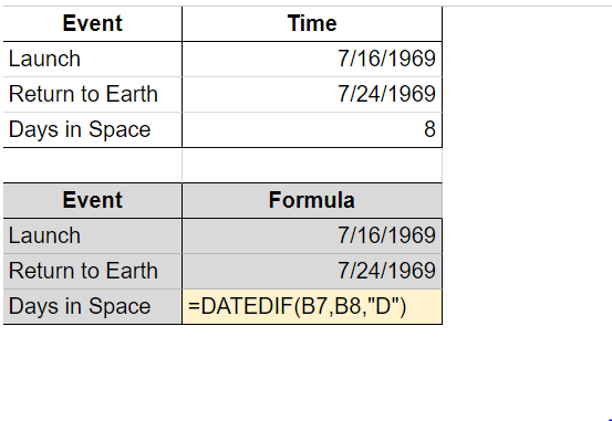
DATEDIF
This function is very simple and it is used when the user needs to calculate the number of days, months, and years between two given dates. So basically this function enables the user to determine the difference between two date values. Following is the syntax for the function.
DATEDIF (start_of_date, end_of_date, unit)
Here, DATEDIF is the name of this date function. Start_of_date refers to the date from where the calculations should start. It may contain a numeric value, a cell consisting of a DATE, or a function translating into a DATE type. End_of_date indicates the date on which the calculations are to end. Likewise, it may also contain a numeric value, a cell consisting of a DATE or a function translating into a DATE type. Units are the text acronyms for the units of time. For example, ‘M’ for a month, ‘D’ for a date, and ‘Y’ represents the year. Following terms should also be known by the users. “Y” indicates the number of years from the start to the end dates. “M” qualifies for the number of total months from the start date to the end date. “D” refers to the total number of days from the start date to the end date.” MD” suggests the total number of days from the start date to the end date after deducting whole months. “YM” represents the total number of months from the start date to the end date after deducting whole years. Now imagine that there is a difference of not more than one year from the start date and end date, then “YD” refers to the number of days from the start date to the end date.
DATEVALUE
This function translates a string with a date represented in text and of known format into a date value. Following is the syntax for this function.
DATEVALUE (date_of_string)
Here DATEVALUE is the name of the function. Date_of_string refers to a string that consists of the textual representation of date but a known format. It should be noted that the input for this function should be a date string and any numeric value in the input will result in an error value. Further, known formats in Google sheets are different in different regions, so if a format i not known in Google sheets then no need to worry. You only have to enter that format into an empty cell sans quotation marks.
DAY
This is another date function and it outputs a certain day from a particular time. It is useful when you are working on time and only require the day from that certain data. The function works in numeric format. The syntax for this function is as follows.
DAY (date)
Here, DAY is the name of the function. The date refers to the date from which you want to take out the day. Date must contain a numeric value, a function providing date type, or a cell with a date. It should be noted that Google sheets refer to date and time as numeric values, therefore this function works only when the input is in number format.
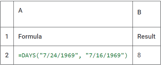
DAYS
Asevident from the name, this date function works for values containing more than one date. Therefore, this function outputs the number of days between two dates. The syntax is as follows.
DAYS (end_of_date, start_of_date)
Here DAYS is the name of the function. End date and start date refer to the two dates between which the user wants to calculate the days. Its format is also numeric. The function outputs the difference between the total number of days between the two dates.
EDATE
This date function enables the user to know a certain date and also a certain number of months before or after that certain date depending on the requirement. The syntax for the function is as follows.
EDATE (start_of_date, months)
EDATE is the name of the function. The start date represents the given date from which the calculation is to be started. Months refer to the number of months the user wants to calculate. It has two types of values; the negative ones refer to the number of months before the start date, while the positive ones refer to the number of months after the start date.
HOUR
Hour is the date function that outputs the hour section of a particular given time. The output is in numeric format. Following is the syntax for the function.
HOUR (time)
Here Hour is the name of this function and time refers to that given bit of time from which the user needs to extract the hour portion. It should be noted that it should be a cell consisting of date/time, a function with a date/time format, or simply a numeric value. This function can also be utilized for other calculations.
MINUTE
This date function outputs the MINUTE section of a given time in a numeric format. For this function to work, this is necessary that the input should be referring to a cell containing a date/time function which returns date/time or containing a serial number of date to be translated by N function. Following is the syntax of this function.
MINUTE (time)
Here, TIME is the name of our function, and time refers to the input. This time contains the required portion of time; minute. As mentioned, Google sheets display date and time as numbers, so it is important to use a numeric format for input. For example, an invalid time format such as MINUTE (12:00:00) will translate as an error. This function extracts the MINUTE section of a given time.
TIME
This time function is also a simple one, it outputs the components of time such as an hour, minute, or a second as TIME. The input of this function should always be in the numeric format as well; otherwise, the function will return an error. Following is the syntax of this function.
TIME (hour, minute, second)
Here, TIME refers to the name of the function. Hour is the input of the hour portion of the given time, a minute is the input of the minute portion of time and finally, the second refers to the input of the second component of time. All the data in numeric format will output TIME. The values of the time that go beyond the valid range of time will automatically recalculate. For example, a time(28, 0, 0) that contains an invalid 28 hours, will be returned as 04:00 AM. Further, TIME will approximate the input which is in decimal form. For example, an hour of 7.25 will return as 7.
Key Takeaways
Google Sheets is among the most powerful and free productivity tools for business people.
GOOGLETRANSLATE is a function that has made understanding texts in different languages possible.
This function is very simple to use and makes the spreadsheet more appealing.
SPARKLINE function enables the users to incorporate mini charts in a single cell of spreadsheets to make them more descriptive and convenient to…
ISBLANK function determines if a cell is empty or not.
ISDATE function determines whether a value contained in a cell is a date or not.
ISMAIL function is used to check whether a certain email address provided in the data is valid or not.
TIMEVALUE
Most of the time, the dates and times in spreadsheets are in the string format, which cannot be directly employed to do any sort of calculations. This TIMEVALUE function is primarily to convert dates and times of string format into time format. Following is the syntax.
TIMEVALUE (time_of_string)
TIMEVALUE is the name of the function. Time_of_string refers to the string containing the text used in the time string. It should be noted that input should be written in the standard form within quotation marks and the time format should be either 12-hour or 24-hour. For example, it should be either 07:38 PM or 19:38. Further, the time string ignores the dates such as the day of the month. So the TIMEVALUE converts simply the time string
Formula
Description
Example Usage
SUM
Adds up a range of numbers.
=SUM(A1:A10)
AVERAGE
Calculates the average of a range of numbers.
=AVERAGE(A1:A10)
MIN
Returns the smallest value in a range.
=MIN(A1:A10)
MAX
Returns the largest value in a range.
=MAX(A1:A10)
COUNT
Counts the number of cells in a range with numbers.
=COUNT(A1:A10)
COUNTA
Counts the number of cells in a range with any data.
=COUNTA(A1:A10)
COUNTIF
Counts the number of cells that meet a specified condition.
=COUNTIF(A1:A10, ">50")
SUMIF
Adds up cells that meet a specified condition.
=SUMIF(A1:A10, ">50")
AVERAGEIF
Calculates the average of cells that meet a specified condition.
=AVERAGEIF(A1:A10, ">50")
IF
Returns one value if a condition is true, and another if false.
=IF(A1>10, "Yes", "No")
IFERROR
Returns a specified value if a formula results in an error.
=IFERROR(A1/B1, "Error")
VLOOKUP
Searches for a value in a range and returns a corresponding value.
=VLOOKUP(A1, B1:C10, 2, FALSE)
HLOOKUP
Similar to VLOOKUP but searches horizontally.
=HLOOKUP(A1, B1:J1, 2, FALSE)
INDEX
Returns the value of a cell in a specified row and column of a range.
=INDEX(A1:D10, 3, 2)
MATCH
Searches for a value in a range and returns its relative position.
=MATCH(A1, B1:B10, 0)
CONCATENATE
Combines two or more text strings into one.
=CONCATENATE(A1, " ", B1)
LEFT
Returns a specified number of characters from the beginning of a text string.
=LEFT(A1, 5)
RIGHT
Returns a specified number of characters from the end of a text string.
=RIGHT(A1, 3)
MID
Returns a specified number of characters from the middle of a text string.
=MID(A1, 3, 2)
LEN
Calculates the number of characters in a text string.
=LEN(A1)
UPPER
Converts text to uppercase.
=UPPER(A1)
LOWER
Converts text to lowercase.
=LOWER(A1)
PROPER
Converts text to proper case (capitalizes the first letter of each word).
=PROPER(A1)
TRIM
Removes extra spaces from a text string.
=TRIM(A1)
TEXT
Converts a value to text in a specified format.
=TEXT(A1, "mm/dd/yyyy")
DATE
Creates a date value.
=DATE(2023, 10, 15)
TIME
Creates a time value.
=TIME(15, 30, 0)
NOW
Returns the current date and time.
=NOW()
TODAY
Returns the current date.
=TODAY()
DATEDIF
Calculates the difference between two dates in various units (e.g., days, months).
=DATEDIF(A1, B1, "d")
EOMONTH
Returns the last day of the month, a specified number of months ahead or behind a given date.
What is 30 Advanced Google Sheets Formulas For Business People?
Google Sheets is among the most powerful and free productivity tools for business people. It enables you to create from simple to more complex spreadsheets, with minimum sophistication, and in many cases, with out of the box formulas, that can handle complex tasks and all this in the cloud, therefore your document is always updated, it can be shared easily with other team members and worked upon.
What is GOOGLETRANSLATE?
GOOGLETRANSLATE is a function that has made understanding texts in different languages possible. This function enables the user to translate certain text from one language to the other, so that has broadened the scope of Google sheets. Following is the syntax.
What is IMAGE?
This function is very simple to use and makes the spreadsheet more appealing. Image is function simply adds a specified image in the cell or range. Following is the syntax.
What is SPARKLINE?
SPARKLINE function enables the users to incorporate mini charts in a single cell of spreadsheets to make them more descriptive and convenient to analyze data . Following is the syntax.
What is ISBLANK?
ISBLANK function determines if a cell is empty or not. This function outputs the value as true if the cell is empty and false if the value is not empty. Following is the syntax.
What is ISDATE?
ISDATE function determines whether a value contained in a cell is a date or not. Following is the syntax.
What is ISMAIL?
ISMAIL function is used to check whether a certain email address provided in the data is valid or not. Following is the syntax.
What is ISERROR?
This function is classified as an information error and it is used to determine an error in a value. Following is the syntax.
What is ISFORMULA?
ISSFORMULA is also classified as an information function. It is employed to determine whether a cell or range contain a formula or not. Following is the syntax.
Gennaro is the creator of FourWeekMBA, which reached about four million business people, comprising C-level executives, investors, analysts, product managers, and aspiring digital entrepreneurs in 2022 alone | He is also Director of Sales for a high-tech scaleup in the AI Industry | In 2012, Gennaro earned an International MBA with emphasis on Corporate Finance and Business Strategy.
Scroll to Top
Discover more from FourWeekMBA
Subscribe now to keep reading and get access to the full archive.


: TSMC's Chip-on-Wafer-on-Substrate Technology")
