Google Drive Service offers several Google products online such as Google Docs, Google Slides, Google Forms, and Google Sheets. Introduced in 2006, Google Sheets is an amazing online spreadsheet application. It is free to use, customizable, and a cloud-based application, which can be accessed anytime and from any device. This application is compatible with Android, macOS, Windows, ChromeOS, and blackberry.
Google Sheets functions like any other spreadsheet tool, but with more advanced features. It is often compared with MS Excel, the time-hallowed giant of the spreadsheet world. However, Excel is primarily an offline program, and Google Sheets being an online and cloud-based application, can be incorporated very well with the other online Google Services.
Google Sheets supports the following spreadsheets files: .xls, .xlsx, .xlsm, .xlt, .xlts .xltm, .ods, .csv, .tsv, .txt and .tab.
Google Sheets is a very efficient tool to create, edit, update, and analyse any kind of information or data. Google Sheets is proving to be a real game-changer in today’s corporate world. The following aspects make Google Sheets the most sought-after application.
Cloud-based
It is a cloud-based application, which means that it saves data on remote servers and can be accessed through the internet at any time, and from any device using an active Google account.
Auto-save
All the data in the Google Sheets is automatically saved online, which means that the data can be retrieved at any time without needing a hard drive. In this way, the reliance on the hard drive becomes minimal while using Google Sheets.
Collaboration in real-time
Collaboration is the most outstanding feature of Google sheets, as this feature allows the teams to work more efficiently saving precious time. Through this feature, several users can add, update, edit, view, and analyse the changes made by the other person and themselves in real-time. Google Sheets offer collaboration at three levels; edit, share, and comment.
Editing
Editing through Google Sheets is one step ahead of all the other spreadsheet programs. As Google Sheets offers collaborative editing in real-time. Through this feature, several people in a team can edit data simultaneously, with the changes being automatically saved on the remote servers. This eliminates the need for mailing the data to several people for editing and revising the details. The Revision History feature enables the edit history to be tracked.
Offline editing
Although Google Sheets is an online application, it also supports offline editing. Meaning that the data can be edited offline on either desktop or through mobile apps. Mobile users need to download Google Sheets mobile app on IOS and android, while desktop users need to download ‘Google Docs offline’ through chrome browser for offline editing.
Comment
Comments can also be made during the editing of the data on Google sheets for adding notes or giving suggestions about some specific information. To comment, you need to click on a cell or several cells for that matter. The comments are shown in the interactive boxes bearing the name and photo of the commenter. After making the required changes the comments can be disappeared by clicking on ‘Resolve’.
Share
Sharing is much simpler and time-saving via Google Sheets. Users can share spreadsheets online with the staff and they can view and edit and update it online. Apart from this, if you do not want your data to be accessed by certain people, data access can be restricted by clicking on the ‘advanced’ option. Then click on ‘prevent editors from changing access’.
Explore
Google Sheets offers the Explore feature since 2016. This feature offers a variety of information based on data the user adds to the spreadsheets. Explore feature is also used to make charts, ask questions, and pivot tables among other things.
Personalize your Google Sheets
Every person uses spreadsheets in his way, using several methods and processes. Google Sheets offers to personalize your Google sheets by using add-ons.
Add-ons
Google Sheets provides add-ons to make graphs and diagrams, to modify and style tables. Click on Add-ons in the menu bar and then click on ‘Get Add-ons’. Choose the Add-on that complements your field of interest.
Basic Google Sheets Terms
To master Google Sheets, there are certain terminologies that need to be understood first. Following are some of the basic terms.
Cell
Google spreadsheets are made from a lot of cells. The horizontal rows and vertical columns intersect and result in a cell. It is a single data point in the spreadsheet. You can make as many as 5 million cells in Google Sheets.
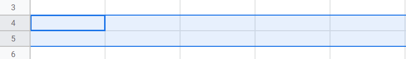
Rows
Rows are horizontal lines, indicated numerically. The rows start from 1 and they are infinite, which means you can make as many rows as you need.
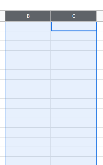
Columns
Columns are vertical lines in a cell. They are indicated alphabetically. They can also be infinite so when alphabets end at Z, the letters go with AA, AB, and so on.
Range
Range refers to a set of selected cells. Range may contain a row, a column, or both. You can also give names to the range depending upon the type of data.
Array
An array is also a sort of range and consists of a table of values, but it is used in a formula. The array can also be named to make it more distinctive.
Function
A function is an in-built operation from the Google Sheets application, it is used to calculate and manage data. There is a function/ formula bar with the ‘fx’ symbol, this space is used to enter data including text, formulas, and functions.
Formula
To calculate data and find out results, the users must apply formulas combining rows, columns, range, etc. For example, there are some, average, and mean formulas that are commonly used in Google Sheets.
Worksheet
It consists of a set of columns and rows making a spreadsheet.
Spreadsheet
It is an entire document containing Google Excel Sheets. Data in a spreadsheet can be represented through text, numeric values, or graphs, etc. There can be more than one worksheet in one spreadsheet.
Google Sheets application is being employed in every field of human activity ranging from making budgets for large and medium-sized businesses to analyzing progress in the corporate world. It is taking over the traditional spreadsheet tools and revolutionizing the ever-changing corporate world.
How to use Google Sheets
Now that we are done with some of the theoretical domains of Google Sheets, now move towards getting to know how to use Google Sheets.
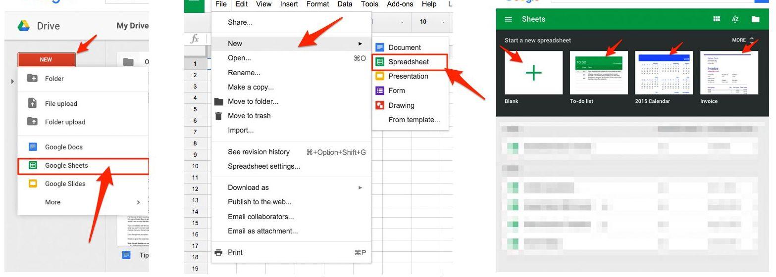
Creating a new Google Sheets Spreadsheet
First, you need to create a new Google Sheets spreadsheet. For this purpose, you need to log into your Google account or if you do not already have a Google account, then create one.
Now there are several ways to create new Google Sheets spreadsheets. One of them will be using your Google Drive app and tapping the plusicon in the bottom right, then select Google Sheets. There are several templates displayed on the top of the page, you can click on the Blank one or you can view the full list of templates in Template Gallery.
It should be noted that a spreadsheet can have multiple numbers of sheets and you can add more sheets to a spreadsheet by using the Plus icon.
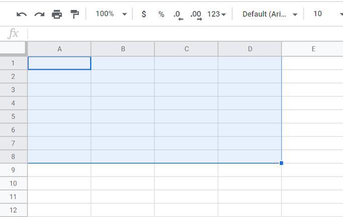
The Google Sheet Editing Window
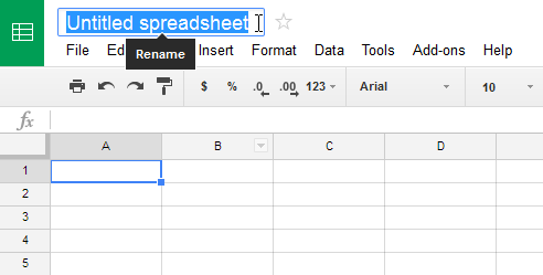
This is how your blank Google Sheet looks like.
Now the spreadsheet is opened and you can give a name to your spreadsheet. For this click on the space named ‘untitled spreadsheet’ and type a name, that fits your purpose. For example, you can name it ‘monthly budget’. Then you can start importing and/or adding data into your spreadsheet.
Understanding Toolbar Icons
To use Google Sheets effectively, you need to understand the icons that are contained in the Toolbar. The Toolbar contains a row of different icons for different functions on the top of the sheet. An image of Toolbar is explained below.
Undo
It is indicated by a curved arrow to the left which enables the user to make corrections and to edit the data.
Redo
Another curved arrow indicates redo but to the right side, it enables you to retrieve something back, which you have undone.
Print
This icon enables the user to directly print the spreadsheet without having to go to the file and then printing it. Therefore, it saves time.
Paint format
It enables the users to set any format for the cells. For this, you have to select a particular format style for your spreadsheet and copy this on format painting. This will change the cursor into a paint roller, enabling you to select the part of the spreadsheet you want for that particular format.
Zoom
This enables the user to get the desired size for the display of your data in cells. For example, if you want to view a cell in detail, you can zoom it in.
Format (as currency $ or percentage %)
Most of the time you need to generate numerical data using currencies or percentages, format (as currency or percentage) icon enables the user to add currency or percentage as data in the range.
Format (decimal position)
There are two options to increase or decrease decimal position, it speeds up the process of changing positions on either side. There are other formats as well, which can be used depending on the type of data you want to enter.
Font and font size
Easily readable fonts make a big difference to make a presentation more appealing. So the font and font size icons enable the user to use the type of font style that is more suitable to your area of interest, also the size of the font can be changed.
Bold, Italics, Underline
These are tools for highlighting the text in the spreadsheets. They help the users to easily mark certain data and easily find it when the need arises. These tools give your spreadsheets an organized look.
Text Colour
It enables the user to change the color of the text as desired. You can use different colors for different items in rows and columns.
Fill Colour
This is an amazing tool, enabling the user to fill the cells with colors. It makes the cells effectively organized and easy to comprehend along with making the spreadsheet more appealing.
Borders
You can choose how you want the borders in the spreadsheet, their color, style, etc.
Merge cells
When you select a range, this feature can be used to merge multiple cells in a range. So, you can merge cells containing data of a particular type, together.
Align
Users do not always require their data to be aligned in a single direction, as different sections of data need to be aligned differently. It enables the user to align the text in the center, left, or right depending on the need.
Vertical Align
It enables the user to align the data in the spreadsheet on the vertical position in the center, top, or bottom.
Text Wrapping
To display the data inside the cell or beyond the cell boundary, you have three options to wrap the data; overflow, wrap, and clip.
Text Rotation
Many times, your data needs to be displayed from different angles instead of a linear position. Text rotation option is there to take care of this.
Insert link
It enables the user to insert links in their spreadsheets for reference. For this purpose, add a word or phrase that is clickable and redirect it to a particular URL. Then click on the paper clip and paste the URL in the popup.
Insert comment
This is very effective for collaboration inside a spreadsheet. Click on the cell you want to add a comment, and this will be displayed in the interactive boxes for all team members to view.
Insert Chart
Often, the users are in need of displaying the data in the form of charts. The insert chart option enables this by clicking onto the range to be converted into a chart. A Chart Editor box is there to enables the user to add the desired kind of chart.
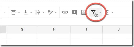
Create Filter
It is an efficient way to start creating filters directly.
Functions
These are very useful in calculating data. Functions contain a drop-down menu with the most used functions like Sum, Average, Mean, and others. There is also a list of functions with categories like Maths, Engineering, and others. Functions help you quickly navigate your data in the spreadsheet without having to memorize all the formulas.
Adding data to Google Sheets spreadsheet
When you open a new spreadsheet, it is blank. You need to add data to it by selecting a cell. The selected cell is surrounded by a blue outline. As soon as you start writing, you will see that a cell at the top left starts being populated with the data that you are entering. You just have to enter the information and no need to double click, as the data is auto-saved on Google Sheets.
When you are done adding the information into the cell you only have to press ‘Enter’ or press ‘TAB’ among other options. Then you can click on the next cell you want to add information into and go.
How to add columns in Google Sheets
To add columns or rows in a spreadsheet, you need to click on the space where you want to add columns/ rows. The desired column/ row will be selected by turning into a blue color, now go to the options menu and right-click, and then you have two options. To add new columns, you need to select Insert Before or Insert After. While for the rows, you need to Insert Above or Insert Below.
How to add columns and rows at the end
Usually, a Google Sheets spreadsheet contains 1000 rows by default. But sometimes it happens that while adding rows you reach the outer edge of your spreadsheet. So the new rows or columns stop adding up. There is an option for adding more rows. But there is a limit to the numbers of rows that can be added.
In the same manner, if you run out of columns, you can always add more. You can go to the menu by right-clicking and add your desired number of columns. If you need multiple numbers of more columns, say you need 5 more columns. Then you can start by selecting the existing last five columns. Then, right-click to select and insert new columns.
Adding multiple sheets
Google Sheets enables the users to organize their data in many sheets. For example, as a teacher, you may want to keep the data about the monthly budget in one sheet, field trips of class students in another one, and complete detail of students in another one. This way, you are spared from having messed up and cluttered spreadsheets. Therefore, the Plus tab on the bottom of your sheet gives you more sheets. There is a tab with several bars on it, next to the plus tab that is called an index button.
How to rename or delete a sheet
To organize the spreadsheets, you need to give proper names to the sheets according to their data. This helps you in sorting information whenever you want. There is an option for renaming your sheet in the menu bar; you can go to the menu by clicking on the small arrow present next to the name (e.g. Sheet 2). There are other options as well in the menu including hide/unhide or delete your sheet.
Adding data via Copy and Paste
Entering all the data manually can be cumbersome and takes time. You can take care of that by using the copy and paste option. There are several ways for that matter. First, you can copy and paste any text or numerical data into a spreadsheet. Secondly, you can copy a table of HTML from a website and paste it into your spreadsheet. Thirdly, you can copy any data from other cells and ranges. Then drag and paste it into the desired cell.
How to Import a file
Importing a file into your Google Sheets spreadsheet is very simple. You can import a file into an existing spreadsheet, or you can also import it into a new spreadsheet depending upon your need. CSVs, XLS, and XLXS are the most commonly imported files on Google Sheets. You can go to file >import> upload menu to import a file from outside of your Google Drive.
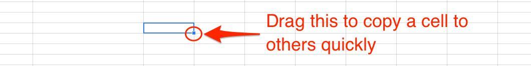
Dragging to copy a cell value
Dragging is needed when you want to copy a cell value across the spreadsheet. You can click on the small blue dot of the selected cell and drag it across or below the spreadsheet when you want to perform different functions.
This feature can be employed for a lot of functions such as copying a cell’s data or formula to neighbouring cells.
Converting Excel to Google Sheets
Excel spreadsheets are the offline competitor of Google Sheets, now sometimes you need to import your Excel spreadsheet into Google Sheets. For this purpose, you need to follow the simple steps. You need to go to ‘file’> ‘import’> ‘upload’ and select the files with the csv, xls, and other type of non-password protected formats.
The imported data automatically gets saved on Google Sheets.
Protecting and sharing data
Now that you have entered data onto your Google Sheets, you are now able to share it with the members of your staff or other people. You can also restrict the permissions to view a certain part of your sheets. So that you can control who can view and edit which part of the data on your spreadsheet. Sometimes the spreadsheets may contain sensitive or confidential data, in such a situation you need to protect your data. Google sheets provide the user with options to protect the data.
Sharing data steps
To share data of your spreadsheet, you can either click on the blue share button or go to ‘file’ > ‘share’. Then enter the email address of the person you want to share your spreadsheet with, add some privacy permissions, like ‘view only’ or ‘edit only’. Some other ‘advanced’ privacy permissions can be employed as well.
Protecting data steps
You can protect your data by proceeding to ‘Data’ > ‘Protected Sheets and Ranges’ and then select the kind of data you want to protect, click ‘set permissions’. You can also make customized settings for a set of people to view your data, and you can set a set of warnings for unauthorized editing of your data.
There are the following permissions for protecting your data.
Viewer: your sheets can only be viewed. Editor: sheets can be changed and edited. Comment: comments can be added/removed in the sheets.
Organizing data in Google Sheets
Google Sheets is a platform that can accommodate a large scale of data in it. This feature is very convenient but sometimes-retrieving data from a huge collection of cells becomes a tiresome business. To counter this, Google Sheets offers several striking options for organizing a vast amount of data.
How to hide data
Google Sheets offers to hide any amount of data on your spreadsheets. It means that you can hide several rows or columns on your spreadsheets. To hide a column, right-click the column you want to hide and select ‘Hide Column’. To hide a row, you can right-click the number of rows you want to hide and then select ‘Hide Row’.
How to unhide data
To unhide data you only need to find arrow icons for the column/ row header bar, hover over the arrows and a box with an arrow will appear. Simply click on the arrow to display the hidden column/row.
Sorting data on Google Sheets
Google Sheets allows you to categorize your data alphabetically, numerically, etc. Sorting helps in clearing the clutter and makes the data more accommodating. Sorting can be done in several ways. For example, you may need to sort data regarding the highest debt to the lowest debt for a private company, or sorting data about the list of golf clubs in a country and so on.
Sorting Range
Sorting range starts from selecting the range that needs to be sorted, clicking Data, selecting Sort Range. Then a dialogue box appears, select ascending or descending. The range is sorted!
Sorting Sheets
Sheets can be sorted alphabetically. You need to have a worksheet with a Header row to identify the name of each column. Although, you need to freeze the header row so that header labels can be exempted from getting included in the sorting.
How to freeze data on Google Sheets
You can freeze your columns and rows on Google Sheets. When you scroll down the rows and columns, freezing them helps in viewing the data more conveniently. On Google Sheets, you can freeze up to 10 rows and 5 columns. Start by selecting the rows or columns you want to freeze by clicking on the row/column numbers. Select View from the menu, float over Freeze rows or Freeze Columns,and select from the drop-down list displayed there.
How to filter data on Google Sheets
The filter option can be used to display only the required set of data from a long list of items. The remaining data will hide and you can easily approach the data you require at a particular time. For example, you may need to have a list of batsmen having participated in all the ICC world cups. However, if you only need to view the batsmen having participated in the ICC world cups since 2011, then you can easily achieve this goal by using the filter. Therefore, the remaining list of batsmen will hide. Start by highlighting the data you want to apply a filter in, then select Data from the menu, then choose filter from the drop-down.
How to format data on Google Sheets
Google Sheets formats most of the data in the spreadsheets directly. Nevertheless, sometimes data needs to format manually. For this purpose, most of the functions can be done using the Toolbar. However, some of the advanced formatting can be done through the format tab. You can use percentage, decimal, currency, and others for numbers. You can also change the decimal positions.
You can change the color, the background of the text. You can also change the font size and font designs. You can also use highlight options bold, italics, strikethrough, or underline to format the text. Therefore, there is a whole world of options and tricks to make your text or data more meaningful and more descriptive when it comes to formatting your Google Sheets spreadsheets.
How to remove formatting
Formatting makes the spreadsheet more convenient to comprehend, but many times you want to remove all formatting from your sheets. For example, when you get data from your colleague, but you want to revamp the entire sheet. This can be done by removing any or all formatting from the cells. The steps are simple. Start by selecting the cells you want to remove formatting from and click Format, then click on the Clear Formatting option.
How to merge Google Sheets
Merging spreadsheets is the most simplistic feature of formatting Google Sheets. Users only have to select ’more than one cells’ and click ‘merge icons’ and you are done. Merging data is a very common activity when you need to analyze perfectly arranged data.
How to use Google Sheets offline
As you are aware that Google Sheets is an online cloud-based application. It means that you are constantly in fear of losing your internet connectivity and thus in turn losing all your Google Sheets data. However, there is no need to panic. As Google Sheets has a feature to be made available offline as well, Not only you can access your Google Sheets offline, but you can also edit it offline. Therefore, that is truly amazing!
Now for Google Sheets to work offline, you need to synchronize your Google account to Chrome because Google Sheets only work with a Chrome browser.
Functions in Google Sheets
Google Sheets offers a large number of Functions in order to do calculations regarding specific values. Each Google Sheets function requires the user to follow a specific order, called Syntax. A basic Syntax requires an equal sign (=), a function name, and an argument. Functions are described in detail below.
ARRAY_CONSTRAIN
This function restricts the size of the input arrays and outputs the specified number of rows and columns of that array. Following is the syntax of this function.
Here the range_of _input is a range of the input data, output_rows is the number of rows that we want in our data, and output_columns is the number of columns that our result may contain. This function is employed along with other formulas when a fewer number of rows and columns are needed in the output.
FREQUENCY
This array function is employed to calculate the frequency of values in a range, known as the one-column range. It gives a vertical array result. The syntax for this function is as follows.
FREQUENCY (data, classes)
Here, data refers to the range or array with the values that are required to be counted. Classes refer to the range with a set of classes. It should be noted that the classes must be sorted to have clarity. The FREQUENCY will output in the form of a specific vertical sized range one greater than classes. An example of the use of this function is given below.
MDETERM
This function is employed to find out the determinant matrix of a given array. Matrix determinant enables the user to calculate the different qualities of the matrix. It should be noticed that the array must be a square matrix comprising only numbers and not any blanks. Following is the syntax for this function.
MDETERM (square_of_matrix)
Here, square_of_matrix represents an array consisting of an equal number of rows and columns; it is the input of this function. A complete matrix should be the input, which will result in a matrix determinant of that specific square matrix. This function can be employed in mathematics to solve system equations in linear algebra. The example is as follows.
MINVERSE
This function determines the multiplicative inverse matrix of a square matrix. This function works specifically with a square matrix, containing numbers only and comprising equal numbers of rows and columns. Following is the syntax for the function.
MINVERSE (square_of_matrix)
Here, MINVERSE is the name of our function; square_of_matix is the input of this function. This function does not work if the array is empty or if it includes text. It enables among other things to calculate a series of simultaneous equations. Following is an example of the use of this function.
MMULT
This array function enables the user to multiply two matrices classified into ranges or arrays. Following is the syntax for the function.
MMULT (matrix1, matrix2)
Here, MMULT is the name of our function. Matrix1 is the name of the first matrix indicated as range or array while matrix2 is the name of the second matrix also indicated as range or array. For the function to work, the standard must be followed. The standard indicates that the columns in matrix1 must be equal in numbers to the rows in matrix2. The output of this function results in the same number of rows as array 1 and the same number of columns in array 2. An example of the use of this function is as follows.
SUMPRODUCT
This array function multiplies 2 or more corresponding entries of equal-sized arrays or ranges and then determines their sum. This function is pivotal in situations where we need to multiply entries across arrays and determine their sum. Following is the syntax for this function.
SUMPRODUCT (array1, [array2, …])
Here, SUMPRODUCT is the name of our function. Array1 refers to the first array or range whose items are to be multiplied with the items of the second array or range via the SUMPRODUCT formula. Array2 refers to the additional arrays or ranges consisting of the same length as the first array or range. Its entries are to be multiplied with the corresponding entries of the first array or range via SUMPRODUCT. Furthermore, SUMPRODUCT can be paired with TRANSPOSE function, resulting in MMULT.
SUMX2MY2
This function enables the user to determine the sum of differences of the entries in two arrays. Following is the syntax for this function.
SUMX2MY2 (array_of_x, array_of_y)
Here, SUMX2MY2 is our function, array_of_x represents the array or range of the entries whose squares are to be minimized by the squares of correlating items in the array_of_y. Then their sum is obtained. On the other hand, Array_of_y represents the array or range of the entries whose squares are to be deducted from the correlating, and then their sum is calculated. An example of the use of this function is shown below.
SUMX2PY2
SUMX2PY2 is an array function that is utilized to find the sum of correlating square entries in two arrays or ranges, which in turn result in sums of their results. It should be noted that the non-numeric values including the text are ignored in the array while using this function. It is used in many statistical problems. The syntax for this function is as follows.
SUMX2PY2 (array_of_x, array_of_y)
Here, SUMX2PY2 is the name of our function. Array_of_x refers to the set of given square entries that are to be added to the square entries of the correlating array or range of array_of_y. While array_of_y refers to the square entries of range or an array whose items are to be added to the correlating square entries of array_of_x.
SUMXMY2
This array function enables the user to determine the sum of squares of differences of values in two given arrays. This function outputs a numeric value. Following is the syntax of this function.
SUMXMY2 (array_of_x, array_of_y)
Here, SUMXMY2 is the name of the function, array_of_x refers to the array or range of the entries that are first minimized by correlating items in array_of_y, then they get squared, and finally, these results are summed up. On the other hand, array_of_y represents the range or array of the entries that will first be deducted from the correlating items of array_of_x, and then they get squared, and finally, these results are summed up.
TRANSPOSE
This array function is very useful when the user wants to relocate the column or rows in an array or range of cells in Google sheets. This function can alter the arrangement of spreadsheets from vertical to horizontal or vice-versa. Following is the syntax of this function.
TRANSPOSE (array_or_range)
Here, TRANSPOSE is the name of the function, while array_or_range consists of the columns and rows of array or range, which are required to be interchanged. This transpose function is very suitable for presentation purposes.
DATE
The DATE function is employed when the user needs to convert the data in the form of DATE from the data that is in the form of a year, month, or day. The syntax for this function is as follows.
DATE (year, month, day)
Here, DATE is the name of this function, a year represents the year section of the date, a month represents the month section of the date, while day refers to the day section of the date. Now certain things should be considered. Firstly, all the input of date should be in numeric form for the function to work properly, otherwise, the output will contain a value error. Further, the DATE is recalculated if the numeric value of the date goes beyond the valid month or day range. For example, the date (2007, 13, 1) which includes the invalid month 13, will be automatically translated into a date of 1/1/2007. Likewise, the date (2007, 1, 32) contains an unreal day of January which will translate into the date of 2/1/2007. The date system that Google Sheets uses is the 1900 date system which starts with the date 1/1/1900.
DATEDIF
This function is very simple and it is used when the user needs to calculate the number of days, months, and years between two given dates. So basically this function enables the user to determine the difference between two date values. Following is the syntax for the function.
DATEDIF (start_of_date, end_of_date, unit)
Here, DATEDIF is the name of this date function. Start_of_date refers to the date from where the calculations should start. It may contain a numeric value, a cell consisting of a DATE, or a function translating into a DATE type. End_of_date indicates the date on which the calculations are to end. Likewise, it may also contain a numeric value, a cell consisting of a DATE or a function translating into a DATE type. Units are the text acronyms for the units of time. For example, ‘M’ for a month, ‘D’ for a date, and ‘Y’ represents the year. Following terms should also be known by the users. “Y” indicates the number of years from the start to the end dates. “M” qualifies for the number of total months from the start date to the end date. “D” refers to the total number of days from the start date to the end date.” MD” suggests the total number of days from the start date to the end date after deducting whole months. “YM” represents the total number of months from the start date to the end date after deducting whole years. Now imagine that there is a difference of not more than one year from the start date and end date, then “YD” refers to the number of days from the start date to the end date.
DATEVALUE
This function translates a string with a date represented in text and of known format into a date value. Following is the syntax for this function.
DATEVALUE (date_of_string)
Here DATEVALUE is the name of the function. Date_of_string refers to a string that consists of the textual representation of date but a known format. It should be noted that the input for this function should be a date string and any numeric value in the input will result in an error value. Further, known formats in Google sheets are different in different regions, so if a format i not known in Google sheets then no need to worry. You only have to enter that format into an empty cell sans quotation marks.
DAY
This is another date function and it outputs a certain day from a particular time. It is useful when you are working on time and only require the day from that certain data. The function works in numeric format. The syntax for this function is as follows.
DAY (date)
Here, DAY is the name of the function. The date refers to the date from which you want to take out the day. Date must contain a numeric value, a function providing date type, or a cell with a date. It should be noted that Google sheets refer to date and time as numeric values, therefore this function works only when the input is in number format.
DAYS
Asevident from the name, this date function works for values containing more than one date. Therefore, this function outputs the number of days between two dates. The syntax is as follows.
DAYS (end_of_date, start_of_date)
Here DAYS is the name of the function. End date and start date refer to the two dates between which the user wants to calculate the days. Its format is also numeric. The function outputs the difference between the total number of days between the two dates.
EDATE
This date function enables the user to know a certain date and also a certain number of months before or after that certain date depending on the requirement. The syntax for the function is as follows.
EDATE (start_of_date, months)
EDATE is the name of the function. The start date represents the given date from which the calculation is to be started. Months refer to the number of months the user wants to calculate. It has two types of values; the negative ones refer to the number of months before the start date, while the positive ones refer to the number of months after the start date.
HOUR
Hour is the date function that outputs the hour section of a particular given time. The output is in numeric format. Following is the syntax for the function.
HOUR (time)
Here Hour is the name of this function and time refers to that given bit of time from which the user needs to extract the hour portion. It should be noted that it should be a cell consisting of date/time, a function with a date/time format, or simply a numeric value. This function can also be utilized for other calculations.
MINUTE
This date function outputs the MINUTE section of a given time in a numeric format. For this function to work, this is necessary that the input should be referring to a cell containing a date/time function which returns date/time or containing a serial number of date to be translated by N function. Following is the syntax of this function.
MINUTE (time)
Here, TIME is the name of our function, and time refers to the input. This time contains the required portion of time; minute. As mentioned, Google sheets display date and time as numbers, so it is important to use a numeric format for input. For example, an invalid time format such as MINUTE (12:00:00) will translate as an error. This function extracts the MINUTE section of a given time.
TIME
This time function is also a simple one, it outputs the components of time such as an hour, minute, or a second as TIME. The input of this function should always be in the numeric format as well; otherwise, the function will return an error. Following is the syntax of this function.
TIME (hour, minute, second)
Here, TIME refers to the name of the function. Hour is the input of the hour portion of the given time, a minute is the input of the minute portion of time and finally, the second refers to the input of the second component of time. All the data in numeric format will output TIME. The values of the time that go beyond the valid range of time will automatically recalculate. For example, a time(28, 0, 0) that contains an invalid 28 hours, will be returned as 04:00 AM. Further, TIME will approximate the input which is in decimal form. For example, an hour of 7.25 will return as 7.
TIMEVALUE
Most of the time, the dates and times in spreadsheets are in the string format, which cannot be directly employed to do any sort of calculations. This TIMEVALUE function is primarily to convert dates and times of string format into time format. Following is the syntax.
TIMEVALUE (time_of_string)
TIMEVALUE is the name of the function. Time_of_string refers to the string containing the text used in the time string. It should be noted that input should be written in the standard form within quotation marks and the time format should be either 12-hour or 24-hour. For example, it should be either 07:38 PM or 19:38. Further, the time string ignores the dates such as the day of the month. So the TIMEVALUE converts simply the time string into a numeric value.
BIN2DEC
This is a function that is used to return a signed binary number as a decimal number. The input for this function should either be the digits 1 and 0 because that is how the binary system functions. The syntax of this function is as follows.
BIN2DEC (signed_binary_number)
Here, BIN2DEC is the function name; signed_binary_number refers to a string, which contains a signed binary value of 10-bit. This signed binary value is converted into a decimal value. A valid binary number always returns as appropriate string input, such as BINDEC (100) and BINDEC (“100”) always return the same result: 4. Further, the input can have a maximum value of 0111111111 and a negative value of a minimum 1000000000.
BIN2HEX
BIN2HEX function as evident from the name outputs a signed binary number as a signed hexadecimal format. The input must always be in binary digits of 1 and 0. Numbers other than these two may return a number error. Following is the syntax.
Here, BIN2HEX is the name of our function. Signed_binary_number is a string containing a signed binary value of 10-bit, which is going to be returned into signed hexadecimal. While significant_digits refer to the number of significant digits required in the result. The positive maximum value for this function is 0111111111 and the minimum negative value is 1000000000. When the user enters a valid signed binary number, then it silently converts to string input. Likewise, if the given significant numbers are less than the required number of digits, then it returns a number error.
BIN2OCT
BIN2OCT is another function of engineering, just like BIN2HEX. But this function is utilized when a signed binary number is required to be returned in signed octal format. Following is the syntax for this function.
Here, BIN2OCT is the name of the function. The signed binary number represents the string of signed binary value of 10-bit that is required to be returned in a signed octal format. Significant digits refer to the number of significant digits required in the output. This function also only works with 2 binary digits of 1 and 0. In this function, two’s complement format is utilized for negative numbers. In this function, the positive value contains 0111111111 numbers at max and 1000000000 negative numbers at a minimum. It is important to note that the octal format should be in place when doing calculations for this function. Significant numbers should not be less than the number of required digits. Otherwise, the number error will be returned.
DEC2BIN
This function is kind of opposite to the function BIN2DEC. T his function outputs a decimal number to a signed binary function. Following is the syntax for this function.
Here DEC2BIN is the name of the function. A decimal number is the input number that must be converted into a signed binary number. There is a maximum of 511 positive and -512 negative values. Significant digits refer to the numbers that must be included in the results. A negative decimal number is ignored.
DEC2HEX
This function is used when a signed hexadecimal format is required to be returned from a decimal number. Following is the syntax.
DEC2HEX (decimal number, [significant number])
DEC2HEX refers to the name of the function. The decimal number refers to the decimal value that the user wants to output into a string format of a signed hexadecimal number. The highest positive value is 529755813887 and the lowest negative value is 549755814888. Significant numbers refer to the number of significant digits that are to be returned. A negative decimal is always avoided.
COMPLEX
This function uses real and imaginary coefficients to produce a complex number. The syntax for this function is as follows.
COMPLEX (real_part, imaginary_part, [suffix])
COMPLEX is the name of the function. The real part refers to the real portion of the coefficient in input, the imaginary part refers to the imaginary portion of the coefficient in input, while the suffix is usually an optional coefficient for the imaginary part.
DELTA
This function is utilized while comparing two numeric entries, and if these entries are equal they output as 1. Following is the syntax.
DELTA (number 1, [number 2])
Delta is the name of the function. Number 1 signifies the first number to be compared, while number 2 in the input is sometimes optional and it signifies the second number to be compared. The second number is 0 by default and when there is no second number then number1 is compared with zero. This function only works for the comparison of numbers.
IMAGINARY
By utilizing this function, an imaginary coefficient of a complex number is returned. Following is the syntax for this function.
IMAGINARY (complex number)
Here, IMAGINARY is the name of our function while a complex number denotes the given number which is to be returned as an imaginary coefficient. The format usually used is either a+bi or a+bj.
IMDIV
This function can be used to divide a complex number with another complex number. The following syntax is used.
IMDIV (dividend, divisor)
Here, IMDIV is the name of the function. The dividend is the complex number in input, which the user wants to divide, while the divisor is the complex number by which the dividend is to be divided. It should be considered that two complex numbers with only the same suffix can be divided (i or j). For example, “6+4i” and “2+3j” cannot be divided.
IMPRODUCT
This function is used to multiply a series of complex numbers, and their result is the output of this function. The syntax for this function is as follows.
IMPRODUCT (first factor, [second factor, …])
IMPRODUCT is the name of the function. The first factor refers to the first complex number or range that is used to find the product, while the second number refers to additional complex numbers that can be added by which the product is calculated. This function like IMDIV function works only when the numbers to be multiplied contain the same ‘i’ or ‘j’ suffixes.
IMREAL
This function is employed to calculate the real coefficients of complex numbers. Following is the syntax.
IMREAL (complex number)
IMREAL is the name of this function. A complex number is the input; this is the number that you want to convert into a real coefficient.
IMSUB
This function output the difference between two complex numbers. Following is the syntax.
IMSUB (first number, second number)
IMSUB is the name of the function. The first number in input refers to the first complex number that needs to be subtracted from the second number. The second number refers to the second complex from which the first number is required to be deducted. The complex numbers that have the same suffixes can be used in this function.
IMSUM
IMSUM function is used when you want to add a series of complex numbers in cells or ranges. The following syntax is followed.
IMSUM refers to the name of the function. The first value refers to the first complex number in range to be added. The second value refers to the additional complex numbers which must be added to the first value. The result is the sum of these complex numbers.
OCT2BIN
OCT2BIN function is used when a signed binary number is to be returned from a signed octal number. The syntax is as follows
Here, OCT2BIN is the name of the function. The signed octal number is the signed value of 30-bit in string format. This is converted into a signed binary number. While a significant number refers to the number of significant digits that are required in the output. The maximum positive value is 777 and the minimum negative value for this function is 7777777000. As evident from the name, the numbers from only 0-7 are valid and the others are returned a number error.
FILTER
This is a filter function. It is employed to filter the source of range, as well as the rows of columns that abide by a particular set of conditions. The following syntax is used.
FILTER (range, first condition, [second condition,…])
FILTER is the name of the function; range refers to the set of cells that are to be filtered. The first condition refers to true or false values within a column or row, which are incongruous with the first row or column of the range, or any other array. While the second condition refers to the optional or additional rows or columns with true or false values evaluating whether correlative rows or columns should be filtered. Conditions of rows however cannot be mixed with that of columns. Therefore, if the conditions are not met the result will return as an error.
SORT
As evident from the name, this function is primarily to sort different items. In the present case, this function is used to sort the rows of array or range into a column or more. Following is the syntax.
SORT here is the name of the column. The range contains the data which is to be filtered through sorting. Sort column refers to a given range having a single column and it must contain the same number of rows as identified in range. Is_ascending contains true or false values representing the order of data arrangement. True values go with ascending order and false values go with descending order. If there is no input value, then the data silently sort in ascending order. Sort column2 and is_ascendind2 are additional and they can be employed to do multiple sorting. It should be noted that only the selected columns are sorted and the others remain unchanged.
UNIQUE
UNIQUE function is used to extract unique rows from the source range and get rid of repeated data. This function makes it convenient to extract unique rows when there is a huge amount of unsorted data. This function outputs the rows in the order of source rows. Following is the syntax.
UNIQUE (range)
Here, UNIQUE refers to the name of function and range refers to the cells of data is sorted in unique rows. If some duplicate rows display in the output then make sure to get rid of any covert text. Format numeric values in their appropriate way, such as currency, etc.
DETECTLANGUAGE
This function is primarily used, as evident from the name, to recognize the language of the text that is used in a certain selected range. Following is the syntax.
DETECTLANGUAGE (text or range)
Here DETECTLANGUAGE refers to the name of the function. Text or range refers to the range in which certain text is present whose language you need to recognize. If there is more than one language in the selected text then the text that comes first is examined.
GOOGLETRANSLATE
GOOGLETRANSLATE is a function that has made understanding texts in different languages possible. This function enables the user to translate certain text from one language to the other, so that has broadened the scope of Google sheets. Following is the syntax.
GOOGLE TRANSLATE (text, [source language, target language])
Here GOOGLETRANSLATE is the name of the function. The input contains text, the source language, and the target language. The text refers to the selected text that you want to translate, source language refers to the language from which you want to translate your text, and target language refers to the specific language in which you want to translate your text. There is a two-letter code for source or target language, which should be written within quotation marks. For example, “en” for English and “ko” for the Korean language.
IMAGE
This function is very simple to use and makes the spreadsheet more appealing. Image is function simply adds a specified image in the cell or range. Following is the syntax.
IMAGE (url, [mode], [height], [width])
IMAGE is the name of the function and url refers to URL of the image which must have a protocol as http: / /. Mode refers to the different sizes that the image can have. These modes are used to compress, crop, or make the custom size of an image. Height refers to the specific height of the image and it can be customized by using mode 4. The width refers to the width of a particular image measured in pixels and it can also be customized.
SPARKLINE
SPARKLINE function enables the users to incorporate mini charts in a single cell of spreadsheets to make them more descriptive and convenient to analyze data. Following is the syntax.
SPARKLINE (data, [options])
SPARKLINE is the name of the function. Data refers to the range or array in which a chart is to be incorporated. Options refer to the additional setting and options for incorporating charts. There is an option ‘charttype’, which contains a list of charts that can be added. The list contains the line, bar, column, and winloss charts. Colors can also be added and changed in the charts.
ISBLANK
ISBLANK function determines if a cell is empty or not. This function outputs the value as true if the cell is empty and false if the value is not empty. Following is the syntax.
ISBLANK (value)
ISBLANK is the name of the function whereas value refers to the cells that are analyzed under this function for whether they are empty or contain data.
ISDATE
ISDATE function determines whether a value contained in a cell is a date or not. Following is the syntax.
ISDATE (value)
ISDATE is the name of function and value refers to the data in the cell which is to be confirmed as a date. It must be ensured to put the date within quotation marks for the function to output properly.
ISMAIL
ISMAIL function is used to check whether a certain email address provided in the data is valid or not. Following is the syntax.
ISMAIL (value)
Here ISMAIL is the name of the function and input consists of a value which is in the form of an email address and is verified through this function.
ISERROR
This function is classified as an information error and it is used to determine an error in a value. Following is the syntax.
ISERROR (value)
ISSERROR is the name of the function and value refers to the value or values to be checked as error(s). This function is used to check all the errors in spreadsheets. If there is an error then the function outputs as true and if there is no error then the function outputs as false.
ISFORMULA
ISSFORMULA is also classified as an information function. It is employed to determine whether a cell or range contain a formula or not. Following is the syntax.
ISSFORMULA (cell)
ISSFORMULA is the name of the function. The input consists of a cell or range to check if that cell or range includes a formula. The function outputs as true if the cell or range contains a formula and it outputs as false if there is no formula.
ISNONTEXT
This function comes in handy when you want to determine whether a cell contains a value, which is not in a textual form such as a date, a number, or time. Following is the syntax.
ISNONTEXT (value)
ISNONTEXT is the name of the function, the input contains value, which is examined as textual or non-textual value. This function outputs as false if there is text in the cell, and true if there is no text found. An empty cell also outputs as a true value but an empty string outputs as a false value. This function is usually used along with IF function.
ISNUMBER
ISNUMBER is the function, which is used to mark numbers in data. Following is the syntax.
ISNUMBER (value)
ISNUMBER is the name of the function and input contains a value that is to be determined as a numeric value. The output is true when there is a number in the cell and false when there is no numeric value. This function is also mostly used along with IF function.
ISTEXT
This function is kind of opposite to the ISNONTEXT function as it is used to determine if the value in the cell is text or not. Following is the syntax.
ISTEXT (value)
ISTEXT is the name of the function and input contains a value, which is checked as text or non-text. If the value returns as true, it is text and if it returns as false then the value does not contain text.
CELL
CELL function is primarily associated with the cells in spreadsheets. This function is employed when the user wants to extract some kind of information regarding a specific cell or cells. Following is the syntax.
CELL (information type, reference)
Here CELL is the name of the function. Information type refers to the specific type of information that needs to be extracted from a cell, while reference means a reference to that specific cell.
FALSE
This is the most basic function in Google sheets. This outputs the value as FALSE. Following is the syntax.
FALSE ()
FALSE is the name of the function. It silently changes FALSE literal to logical FALSE.
OR
OR function is a common function that outputs as true if given arguments are true logically. It outputs as false if the given arguments are logically false.
OR (logical expression1, [logical expression2,…])
OR is the name of the function. Logical expression 1refers to the cell, which contains a logical value true or false. Logical expression 2 refers to the additional and optional logical true or false values. All the numbers are logically true except zero, which is false logically.
TRUE
This function is directly opposite to the FALSE function. This determines the value as logically TRUE. Following is the syntax.
TRUE ()
TRUE is the name of the function. Google sheets mostly change TRUE literal to TRUE logical value.
CHOOSE
This is a lookup function. It outputs the chosen element from the index made from a list. Following is the syntax.
CHOOSE (index, choice1, [choice2])
CHOOSE refers to the name of the function. Index refers to 29 options from which to choose. Negative index, zero and more than the choices is returned as number error. Choice1 refers to the cell or value, which is requested and returned in the output. Choice 2 is any other optional value to choose.
COLUMN
COLUMN function is used when you want to know the number of a certain column in a given cell or range. Following is the syntax.
COLUMN (cell reference)
COLUMN is the name of the function. Cell reference refers to the column in which the number is requested. By default, A column corresponds to 1.
ROWS
ROWS is a function that can be used to determine the number of rows that are present in a certain cell or range. Following is the syntax.
ROWS (range)
ROWS refers to the name of the function and range is the input that contains the row required to be counted. For example, ROW (D4) outputs as 4 because D4 is the fourth row in the spreadsheet.
ABS
ABS function is used when the absolute value of a number is requested. Absolute value is always positive, as if there are any negative numbers, then they are converted into positive ones. Following is the syntax for this function.
ABS (value)
ABS is the name of function and value refers to the certain value of which you need to determine absolute value.
EVEN
EVEN is a MATH function that is employed when you need to round up a certain number to the nearest even number. Following is the syntax.
EVEN (value)
EVEN refers to the function, value refers to the certain value which is to be rounded off to the nearest even integer. A negative value rounds off to the nearest negative even value.
GCD
GCD is short for the greatest common divisor. It outputs the greatest common divisor or one or multiple integers. Following is the syntax.
GCD (first value , [ second value,…]
GCD is the name of the function; the first value contains the cell or range whose factors are used in the calculation to find the greatest common divisor. The second value refers to any additional values that need to calculate the greatest common divisor. Decimal values are reduced.
IMPOWER
IMPOWER function is used to output a complex number that is raised to a power. Following is the syntax.
IMPOWER (complex base, exponent)
IMPOWER is the name of the function, complex number refers to that certain complex number that is raised to an exponent; an exponent is always a number to which the complex number is raised.
IMSQRT
This function is simply used to calculate the square root of a complex number or many complex numbers. Following is the syntax.
IMSQRT (complex number)
IMSQRT here refers to the name of the function. It contains the input in the form of a complex number of which the square root is returned in the output. Usually, there is no square root of a negative real number.
ISEVEN
This function is used to determine if a given value is even. Following is the syntax.
ISEVEN (value)
ISEVEN refers to the name of the function, value refers to the value that is requested to be determined as even. If the value is even, output returns as true, otherwise it returns as false. This function is used mostly along with IF function.
Key Takeaways
It is a cloud-based application, which means that it saves data on remote servers and can be accessed through the internet at any time, and from any…
All the data in the Google Sheets is automatically saved online, which means that the data can be retrieved at any time without needing a hard drive.
Collaboration is the most outstanding feature of Google sheets, as this feature allows the teams to work more efficiently saving precious time.
Editing through Google Sheets is one step ahead of all the other spreadsheet programs.
Although Google Sheets is an online application, it also supports offline editing.
Comments can also be made during the editing of the data on Google sheets for adding notes or giving suggestions about some specific information.
Sharing is much simpler and time-saving via Google Sheets.
LOG
LOG is short for Logarithm and it results in the logarithm of a given base. Following is the syntax.
LOG (value, base)
LOG is the name of the function. The input contains a value and a base. Value refers to a certain number of which logarithms is requested, and the base is employed to calculate the log of that number. The value of which logarithm is requested should be positive.
Final Word
To sum it all up, Google Sheets is an amazing tool, a collaboration platform and a comprehensive cloud-based application. It has enabled individuals, businesses and organizations around the world to gather, analyse and manage their data in a revolutionary way. While this extensively covers a lot that there is to Google Sheets, there is much more that can be learned and many use cases to be explored. At the end of the day, it boils down to the needs of the individual or the organization using Google Sheets to decide how they can leverage its functionalities and capabilities to bring innovation to their data and services.
Frequently Asked Questions
What is How To Use Google Sheets?
Google Drive Service offers several Google products online such as Google Docs, Google Slides, Google Forms, and Google Sheets. Introduced in 2006, Google Sheets is an amazing online spreadsheet application. It is free to use, customizable, and a cloud-based application, which can be accessed anytime and from any device.
What is Collaboration in real-time?
Collaboration is the most outstanding feature of Google sheets, as this feature allows the teams to work more efficiently saving precious time. Through this feature, several users can add, update, edit, view, and analyse the changes made by the other person and themselves in real-time. Google Sheets offer collaboration at three levels; edit, share, and comment.
What is Offline editing?
Although Google Sheets is an online application, it also supports offline editing. Meaning that the data can be edited offline on either desktop or through mobile apps. Mobile users need to download Google Sheets mobile app on IOS and android, while desktop users need to download ‘Google Docs offline’ through chrome browser for offline editing.
What are the personalize your google sheets?
Every person uses spreadsheets in his way, using several methods and processes. Google Sheets offers to personalize your Google sheets by using add-ons.
How do you create a new Google Sheets Spreadsheet?
First, you need to create a new Google Sheets spreadsheet. For this purpose, you need to log into your Google account or if you do not already have a Google account, then create one.
What is the google sheet editing window?
Now the spreadsheet is opened and you can give a name to your spreadsheet. For this click on the space named ‘untitled spreadsheet’ and type a name, that fits your purpose. For example, you can name it ‘monthly budget’. Then you can start importing and/or adding data into your spreadsheet.
What is Toolbar Icons?
To use Google Sheets effectively, you need to understand the icons that are contained in the Toolbar. The Toolbar contains a row of different icons for different functions on the top of the sheet. An image of Toolbar is explained below.
What is Adding data to Google Sheets spreadsheet?
When you open a new spreadsheet, it is blank. You need to add data to it by selecting a cell. The selected cell is surrounded by a blue outline. As soon as you start writing, you will see that a cell at the top left starts being populated with the data that you are entering. You just have to enter the information and no need to double click, as the data is auto-saved on Google Sheets.
Gennaro is the creator of FourWeekMBA, which reached about four million business people, comprising C-level executives, investors, analysts, product managers, and aspiring digital entrepreneurs in 2022 alone | He is also Director of Sales for a high-tech scaleup in the AI Industry | In 2012, Gennaro earned an International MBA with emphasis on Corporate Finance and Business Strategy.
Scroll to Top
Discover more from FourWeekMBA
Subscribe now to keep reading and get access to the full archive.